class: title-slide <div style="min-height:100%; height:100%; width:100%;"> <div style="height:65%; width:100%; background-color:clear;"> </div> <div style="width:100%; background-color:#fee600;"> <table style="width:100%; border:0px"> <tr> <td style="width:20%; vertical-align:middle;"><img src="http://www.philipclare.com/img/unsw logo.jpg" style="width:100%;"></td> <td style="width:80%; vertical-align:middle;"><h1>Robust causal inference using non-randomized longitudinal data</h1></td> </tr> </table> </div> <table style="width:100%; border:0px"> <tr> <td style="width:20%; vertical-align:top;"><br></td> <td style="width:80%; vertical-align:top;"><h3>Philip Clare</h3></td> </tr> </table> </div> --- # Acknowledgements Funding: - I receive an RTP Scholarship from the Australian Government and a Scholarship from NDARC - NDARC receives funding from the Australian Government Department of Health Thanks to my PhD Supervisors: Tim Dobbins, Richard Mattick and Raimondo Bruno. --- # Overview 1. Background; 1. Bias in causal inference; 1. Assumptions in causal inference; 1. Methods for causal inference; 1. Targeted maximum likelihood estimation; 1. TMLE Examples; 1. Conclusions; 1. 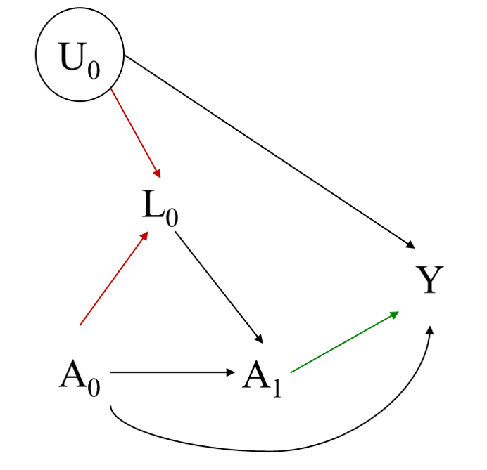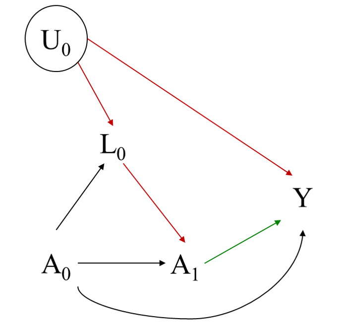References; --- # Background - Causal inference at its simplest: - "the difference in a given outcome, based on some prior event, compared with what would have happened had that event not occurred" - RCTs are, and will remain, the gold standard - There are times when RCTs aren't possible - Causal inference is possible without randomization - It just requires more caution --- # Bias in causal inference - General to all observational studies - Selection bias - Confounding - Collider bias - Measurement error - Specific to longitudinal analysis - Loss to follow-up - Exposure affected time-varying confounding --- # Bias in causal inference .center[  ] --- # Bias in causal inference .center[  ] --- # Bias in causal inference .center[  ] --- # Assumptions in causal inference - No interference - Consistency - Positivity - No unmeasured confounding --- # Methods for causal inference - Propensity score matching (PSM) - Marginal Structural models (MSM) - G-computation - Doubly-robust methods (DR) --- # Methods for causal inference - Doubly-robust methods (DR) - At their simplest: DR methods are those that provide consistent estimates even when one of either the propensity or outcome models are estimated consistently 'Simple' DR methods: - adjusted IPTW - IPTW weighted - G-computation - A-IPTW - Similar to IPTW, but adjusts the IPTW estimate by a function of the outcome model - There is some discussion about the best approach for this in terms of estimating the models --- # Targeted maximum likelihood estimation - TMLE is a targeted substitution estimator that treats everything except the target estimand as 'nuisance' parameters - TMLE involves: - estimating an initial conditional expectation of an outcome using maximum likelihood, - estimating the propensity score, - using the propensity score to create a 'clever' covariate h, and - updating the outcome model based on a function of the initial estimates and the clever covariate --- # Targeted maximum likelihood estimation - This can be repeated if necessary, and will iterate to the target parameter .center[  ] - 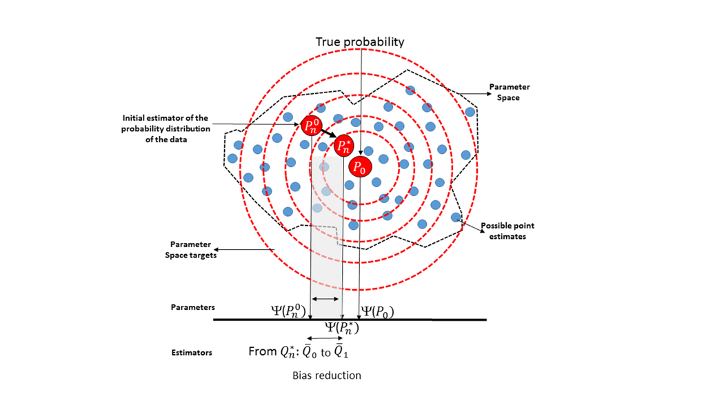However, it has been shown that most common effect measures can be estimated in one iteration --- # Targeted maximum likelihood estimation - Because it is a substitution estimator that doesn't use the parameters of the initial models, TMLE is commonly estimated using ensemble machine learning - The ensemble machine learning algorithm 'Super Learner' was developed in parallel with TMLE - The packages 'tmle' and 'ltmle' in R both call 'SuperLearner' by default --- # Targeted maximum likelihood estimation - TMLE is relatively new - There are a number of areas of ongoing investigation regarding the performance: - Balance SuperLearner: an adaptation of the SL algorithm optimized for balance rather than accuracy of prediction - Collaborative TMLE, which uses a loss function based on Q to fluctuate the nuisance parameter, instead of a loss function of the nuisance parameter itself. 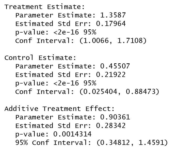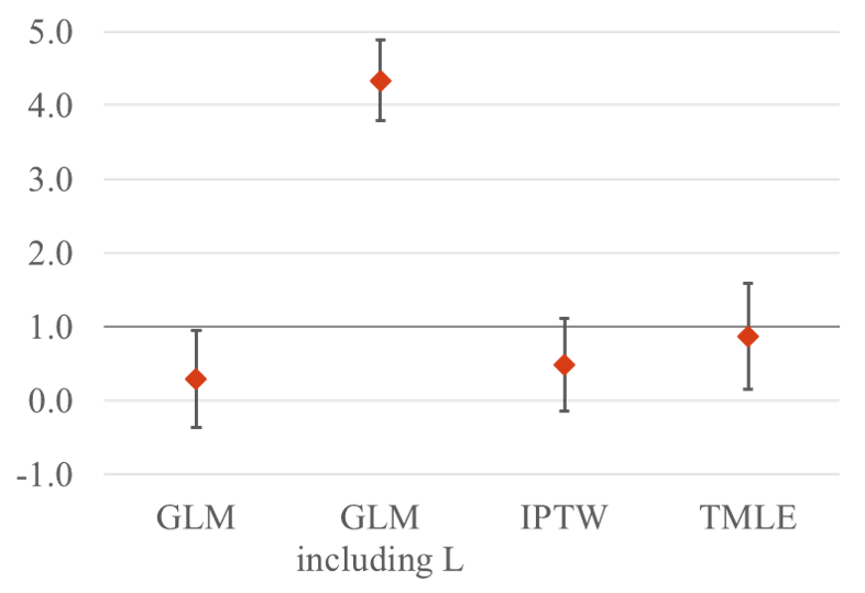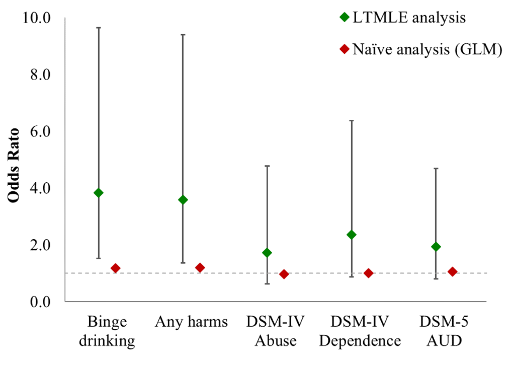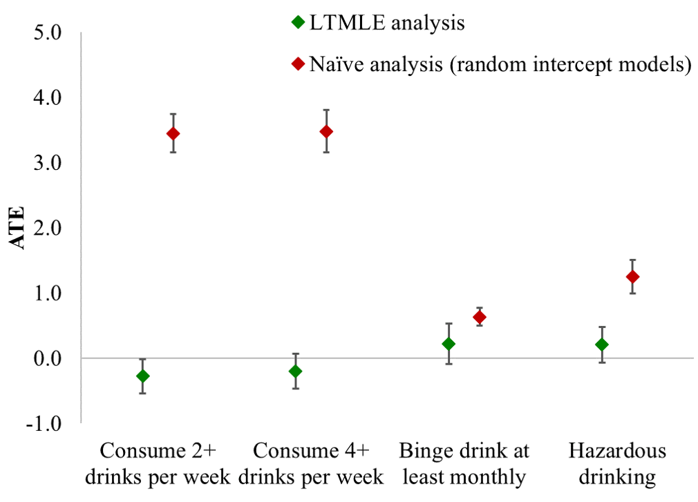C-TMLE can be a consistent estimator even when both models are misspecified --- # TMLE Examples - Random data following the DAG from earlier - True parameter is: .center[ `\(Joint = 0.5×A_0 + 1.5×A_1 - 1.0×A_0×A_1 = 1.0\)` ] .center[  ] --- # TMLE Examples .center[  ] --- # TMLE Examples .center[  ] --- # TMLE Examples .center[  ] --- # TMLE Examples .center[  ] --- # Conclusions - Unbiased causal inference is possible in non-randomized studies - There are methods to deal with bias - Newer methods are more robust - Even for analysis of association, bias is an issue that can be addressed by these methods - Markdown for a TMLE tutorial currently under review at Statistics in medicine: https://github.philipclare.com/tmletutorial --- # References .small[ 1. Clare PJ, Dobbins TA, Mattick RP. Causal models adjusting for time-varying confounding-a systematic review of the literature. Int J Epi. 2019;48(1):254-265. 1. Robins JM. Marginal Structural Models. 1997 Proceedings of the American Statistical Association, Section on Bayesian Statistical Science. 1998:1-10. 1. Robins JM. A new approach to causal inference in mortality studies with a sustained exposure period-application to control of the healthy worker survivor effect. Mathematical Modelling. 1986;7(9):1393-512. 1. Bang H, Robins JM. Doubly robust estimation in missing data and causal inference models. Biometrics. 2005;61(4):962-72. 1. Van der Laan MJ, Rubin D. Targeted Maximum Likelihood Learning. Int J Biostat. 2006;2(1). ]